Vagrants

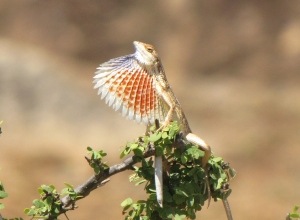
Red-Footed Falcon. Photo by Ariefrahman/Ron Knight from Wikipedia — Red-Footed Falcon. Photo by Ariefrahman/Ron Knight

Here is a piece I wrote last week for The Hindu BLink on vagrant birds. It’s part of a themed issue on the importance of One, including pieces about how single individuals navigate the world, and the impact they have while doing so. This is the first time I’ve written about an assigned topic, and the time frame from assignment to article was three days, so my method of writing diverged a bit from normal.

I knew nothing about vagrant birds two weeks ago. But the advantage of working in a diverse department of biologists, one that includes a natural history museum, is that I could simply walk upstairs to chat with the ornithologists, asking them what they think about vagrant birds. Most had fascinating stories of encounters with vagrants, some of which went into the piece (all crowded into one sentence towards the end).

I had a sense that birders were often excited about spotting vagrants, but wasn’t quite sure why. In my conversations, however, I learnt about “twitchers”–birders who chase down species to spot them and add them to a list of some kind. This could be a life list, a country list, a state list, a county list, and the more bird species are on the list, the better. But birders who care about more than ticking a species off a list are also fascinated by vagrants: one person described being impressed by the distance that vagrants travel, by just how far off course they managed to get. Another viewed vagrants as providing insight into the process of migration, sort of like how disease can offer insight into how the body functions normally. Both cited a specific example as illustrating these reasons: a Red-Footed Falcon, usually confined to Europe, that made its way to the East Coast of the U.S., the first time the species was spotted in the Western Hemisphere! This particular bird drew in many, many birders, each with their own reasons for wanting to see this special vagrant. The bird also got lots of media attention.

Birders watching the Red Footed Falcon at Martha's Vineyard. Photo by Julian Hough at surfbirds.com — Birders watching the Red Footed Falcon at Martha’s Vineyard. Photo by Julian Hough at surfbirds.com

A second thing that came up in my conversations that I found interesting was the feeling of uncertainty that sometimes surrounds the spotting of a vagrant. Some birds, like this falcon, stay in one place long enough that they can be identified and re-identified until everyone’s certain what species they belong to. But other birds aren’t quite as cooperative, flying off before their identity can be confirmed, before even a photograph can be snapped. And because vagrants are, by definition, in an unexpected location, it can be hard to convince someone else that you spotted a vagrant. There is always a similar looking bird that one expects to find in the that location, leaving the birder with just their own conviction that they saw something extraordinary.

Thanks to all the birders (Cassie Stoddard, Maude Baldwin, Peter Wilton, Alison Schultz, Jeremiah Trimble, Gabe Gartner, and Gautam Surya) who contributed their thoughts on vagrants!

A Weird Thing About Principal Component Analysis Loadings…

So if you’re an ecologist of any sort, you’ve probably used and definitely come across principal component analyses (PCA). These analyses are a way to compress a large number of correlated variables into a few variables that capture most of the variation seen in the larger dataset. This is achieved by constructing linear combinations (called principal component axes) of the original variables with a couple of constraints:

1. The first linear combination should capture as much of the variation in the dataset as possible

2. Subsequent linear combinations should also be as variable as possible, and must be uncorrelated with the previous linear combinations.

For example, imagine that you’re measuring body dimensions of frogs. Individuals that are longer in length probably also have longer legs and larger heads. For such a dataset of morphological variables, the first principal component axis is usually a linear combination in which the coefficients of each variable in the linear combination are roughly equal in magnitude and have the same sign. Such an axis is usually interpreted as measuring the overall “body size” of the organism. Subsequent axes are then interpreted as different body shape variables, some of which can be biologically interesting. For instance, in datasets that include morphological measurements of both males and females, a shape axis might point to differences in dimensions between the sexes.

Here’s a simple mathematical representation of a PC axis from a PCA with three variables:The vector of coefficients, a, describes the weight given to each variable in constructing the principal component axis, and is therefore crucial to interpreting the biological relevance of the axis being constructed. I’ve always been taught that this vector is referred to as the loadings of the principal component axis on the original variables in the dataset. But my advisor, Jonathan Losos, recently realised that what he (and many other people) refers to as loadings is entirely different than what I (and many other people) call loadings. What he calls loadings are instead the correlations between the principal component axis X₁ and the original variables x₁, x₂, and x₃. It isn’t entirely clear when or how this change in definition came about, but it might be at least partly attributable to the advent of the functions prcomp and princomp, implemented in the widely used statistical software R, which carry out PCAs and report the first but not the second definition of loadings.

How different is the information conveyed by the two different definitions of loadings? For highly correlated datasets, such as the ones we’re most likely to conduct PCA on, they don’t seem vastly different. This claim is based on my calculations of both definitions of loadings for three or four morphometric datasets I have lying around–the two loadings were perfectly correlated for each dataset. But for less correlated datasets, the answer might be different. Here is a graph of the relationship between the two types of loadings (described as “coeff” and “cor” respectively below) for PCAs conducted on randomly generated normal variables:

Someone more mathematically savvy than me should calculate this relationship explicitly for a number of datasets with varying correlation structures, so that we can assess whether this shift in definition of PCA loadings has implications for how we’ve been interpreting the biological relevance of these axes. Given how widely used PCAs are, it’s well worth knowing what these implications might be.

Being Explicit about Resources will (has?) Revolutionize(d) Sexual Selection

I promised a long time ago to write about the talks at SICB 2014 that changed the way I think about sexual selection. I managed one post about signalling in paper wasps before getting sidetracked into writing about other things. It’s now been far too long since the meeting for me to remember enough about Nathan Morehouse‘s talk in the “Stress, Condition, and Ornamentation” symposium to deliver an accurate summary of the empirical work he presented (unfortunately my notes are as dreadful as my memory). So instead I’m going to explain the concepts as best I remember them and refer you to a paper–Morehouse et al. (2010)–that address some of the same issues as the talk.

What Morehouse demonstrated clearly and memorably in his talk is that our usual framework of sexual selection is terrible at making predictions. Imagine that you are studying a species where males have a large, colourful ornament (a Sitana perhaps?), and suppose that you’ve measured some index of condition (say parasite load), as well as some index of investment in the ornament (size or colour, for example) for these males. Now imagine that you find that parasite load decreases with increased ornament investment. Can you explain this? Sure! Individuals in this species must vary in some underlying “condition” variable, and males in better condition can invest in both their immune system (leading to fewer parasites) and their expensive ornaments.

But imagine you found that parasite load was positively correlated with investment in the ornament. You could explain this too, by positing that males who invest heavily in their ornaments don’t have enough resources left over to also invest in immunocompetence. That we can explain two diametrically opposite results using the same framework suggests that we need to reconsider and clarify the processes underlying the patterns we seek to explain.

Morehouse traced this contradiction to the imprecision with which we think about resource acquisition and allocation–how creatures obtain particular resources from their environment, and how they then invest those resources in particular traits. The scenario posed above could easily be clarified if we knew what nutrients were responsible for ornament quality and parasite resistance, whether these nutrients were limited in the environment, and whether there was variation among individuals in their ability to acquire these nutrients. Imagine two individuals that differ in ornament quality: if we know that, in this species, individuals vary in their abilities to acquire resources but not in allocation strategies, we’d expect that the male with the better ornament to also have a lower parasite load. In contrast, if individuals in this species don’t vary in resource acquisition strategies but instead differ in how they divide up their resources among different body parts, we’d expect the flashier male to have more parasites than the drab male. In real life, individuals will probably vary in both acquisition and allocation, but this variation is potentially quantifiable, and therefore can be used to make predictions about the relationships we expect to see between ornaments and parasites.

In his talk, Morehouse presented some results on nitrogen acquisition and allocation to UV reflective patches in male cabbage butterflies that demonstrated the power of this approach. Consider this post a teaser for future coverage of the butterfly story. He made the case for holometabolous insects–insects that metamorphose from larvae to adults–as particularly good systems in which to ask questions about resource acquisition vs. allocation, because the two processes are completely separated between the larval and adult stages. Larvae are little eating (=resource acquisition) machines, whereas all the allocation to reproductive structures and ornaments only occurs at metamorphosis.

I’m not yet sure how widely this framework of being explicit about resources has been adopted in studies of sexual selection. Morehouse et al. (2010) has been cited roughly 20 times, and a quick scan of the titles of these papers suggests that the field is well on it’s way to being more nutritionally explicit and, one hopes, more predictive.

Cabbage White Butterfly. Photo by J.M. Garg